
There will be occasions when the decimal places that Excel ordinarily calculates to are not necessary; we are only interested in the non-decimal part of the calculation. For example, if our calculation is to determine how many full-time staff members or machines are required to do a job, then we are unable to have half a person or half of a machine (at least without it risking getting messy!)
A “sort of” solution with formatting
There is a temptation to use some of Excel’s formatting tools to help with this, but they may cause us problems down the line.

If we use the “Decrease Decimal” button
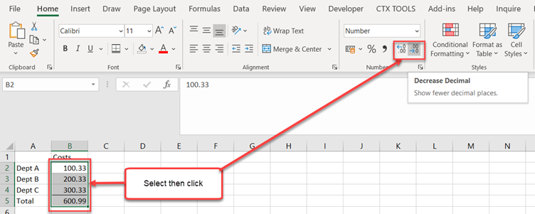
…(or Format to zero decimal places)…
- Select Data
- Click Expand button
- Select Number Tab
- Select Number Format
- Type in number of decimal places (or use the spinner)
- Click OK

We will end up with something that “looks” right…

However, if you look at the total, something has clearly gone wrong and, in the Formula Bar, the original value is still there…

So, we need a better solution and that is provided by the ROUND function.
Using the ROUND Function
Consider this example…

Cell C4 contains the formula C2/C3. As you can see, the result is displayed using a large number of decimal places. We are going to redo this formula and use the Round function to display the result with no decimal places.

First, we click on the cell C4 and press the Del key to delete the cell contents.
Then, from the Formulas tab and within the Function Library group we click on the Math & Trig button. From the drop-down list displayed we select the ROUND function (this may involve scrolling down the list to see this function).

The Function Arguments dialog box is displayed.

In the Number section of the dialog box, we enter the formula C2/C3.
In the Num_digits section of the dialog box, enter 0.

Click on the OK button and you will see the following.

If we click on cell C4, we will see the function syntax displayed in the Formula Bar: =ROUND(C2/C3,0)
This is now the number 365 exactly.
Associated Functions
Earlier we considered the possibility of calculations to determine how many employees or machines were needed.
In determining the value to be shown, the ROUND Function “looks to the right” and if the first digit to the right is 5 or higher, it rounds UP with 4 or lower resulting in rounding down.
However, if our calculation results in the result that (without rounding) we need 6.34 employees or machines, then using ROUND, we will see that we need 6 which would result in us having too few people or machines.
This is where the associated functions of ROUNDUP and ROUNDDOWN can be used. Other than a different function name, the syntax (Number and Num_digits) is identical. However, ROUNDUP always rounds up and ROUNDDOWN always rounds down irrespective of the value of the “first digit to the right”.