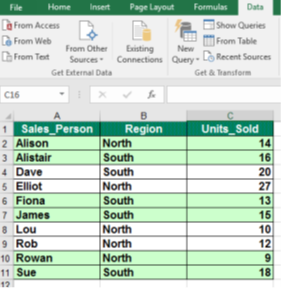
When we have a list of data, sometimes it can be quite difficult to extract information from it quickly and efficiently. However, provided that we’ve the right sort of information in the various columns of our list, then we can make a start by using Excel’s AutoFilter.
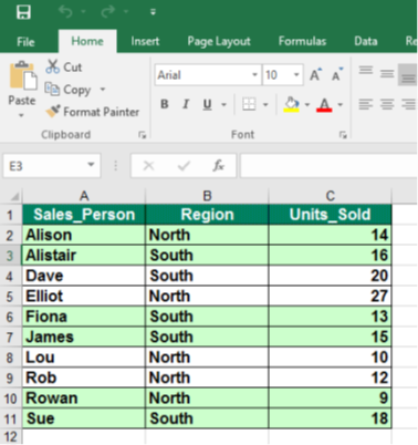
Applying the AutoFilter
Click on any cell within the list.
Click on the Data tab and within the Sort & Filter group click on the Filter button
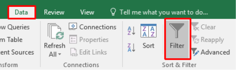
Each of the headings in our list will now have a filter arrow at the right-hand edge of the cell. We can click on these down arrows to apply filters to the data.

Using the AutoFilter
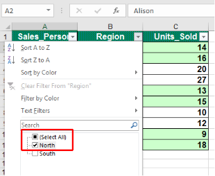
To see only sales relating to the North region, click on the down arrow in the Region column and click on the check box next to Select All.

The drop down list will now look like this:
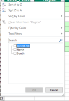
Click on the North check box.
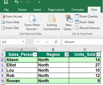
You will then only see sales relating to the North region.
Resetting the AutoFilter
To remove the filter and see all the regions, click on the down arrow in the Regions column and re-click on the Select All.
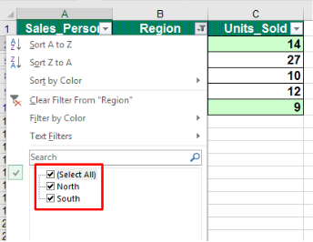
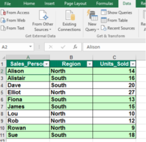
You will now see all the regions displayed again.
Applying a Custom AutoFilter
In addition to simple filters based on matching to specific values within a column, we can also apply a Custom Filter to enable us to look at a range of values…
Let’s say you want to only display details for salespeople that have sold more than 11 units. Click on the down arrow in the Units Sold column and select the Number Filters command. From the sub-menu displayed select Custom Filter.

This will display the Custom AutoFilter dialog box.
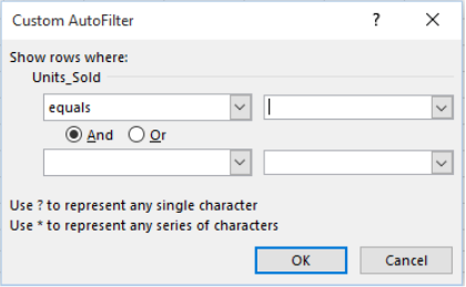
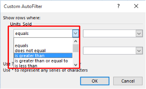
Click on the down arrow next to the Units Sold section and select ‘is greater than‘.
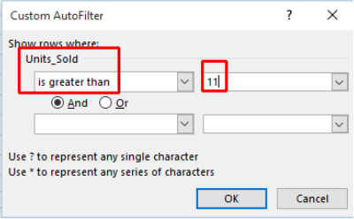
In the box to the right enter the number 11. The dialog box will now look like this.
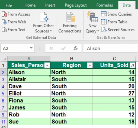
Click on the OK button and the filtered list will look like this.
Using AutoFilter to perform multiple queries
You can use AutoFilter to perform a query using multiple criteria. For instance, you can filter the list to only show sales within the North region of more than 11 units.
So, first of all, we select the North Region…
Click on the down arrow in the Region column and click on the check box next to Select All.
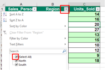
Click on the check box next to North.
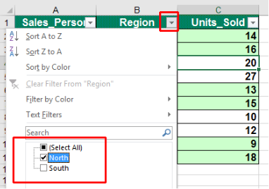
Your table will now only show sales relating to the North region.
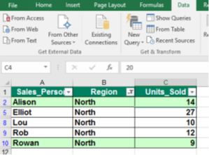
Now we need to restrict the number of units sold…
Click on the down arrow in the Units_Sold column and select Number Filters. From the sub-menu menu displayed click on Custom Filter.

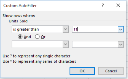
The Custom AutoFilter dialog box is displayed. Click on the down arrow in the Units_sold section of the dialog box, and select is greater than.
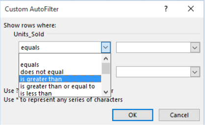
Type the number 11 into the text box in the right hand section of the dialog box. The dialog box should now look like this:
Click on the OK button to apply the filter.
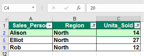
You will now only see data relating to the North, for sales over 11 units.
Top 10 AutoFilter
Slightly mis-named the “Top 10” AutoFilter allows you to select the “Top” or “Bottom” values in terms of the actual number of items or in percentage terms and, whilst the default is 10, you have the option of setting this to any value.
So, with the AutoFilter applied to our list…
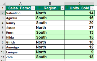
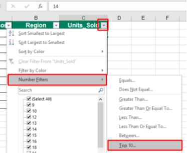
We click on the down arrow in the Units_Sold column and from the drop down menu displayed click on Number Filters. From the submenu displayed click on Top 10.
The Top 10 AutoFilter dialog box will be displayed.
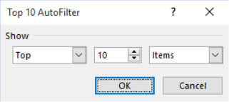
We can then, for example, change the Top value to 5, as illustrated:
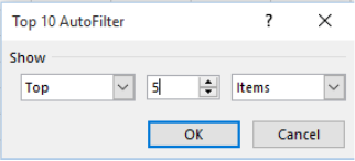
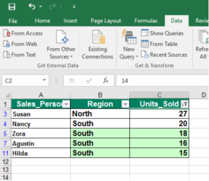
Click on the OK button and you will see the top 5 entries listed, as illustrated:
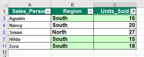
You can then sort these in descending order. To do this click on the AutoFilter down arrow in the Units_Sold column and click on the Sort Largest to Smallest command.
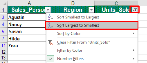
The sorted data will look like this:
Removing all AutoFilters from a worksheet
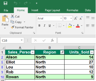
An AutoFilter has been applied to the list within this worksheet.
Click within the data table.
Click on the Data tab and within the Sort & Filter group click on the Filter button
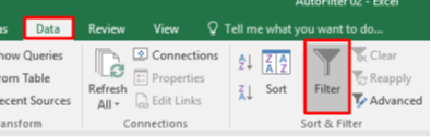
This will remove all filters and display all records.